Bayes-UCB algorithm

Today, a colleague of mine presented a paper called Identifying general reaction conditions by bandit optimization during a Journal club. There are lots of things to say about the chemistry the authors are trying to tackle, but I had never heard of the algorithm before and had a hard time pretending I understood the paper as a result.

Here’s a summary of what I learned about the Bayes-UCB algorithm.

Reminder of multi-armed bandit

The multi-armed bandit problem is a classic decision-making scenario where a gambler must choose between multiple slot machines (or “arms”), each with an unknown payout probability, to maximize their total reward over time. The challenge lies in balancing exploration (trying different arms to gather information about their payouts) and exploitation (selecting the arm known to yield the highest reward).

This problem models real-world situations where one must make a series of decisions under uncertainty, such as clinical trials or online advertising. In the paper, the authors are looking for chemical reaction conditions (ligands, bases, activators, solvents, temperature…) that return the best yield across a batch of reactions. In their study, the arms are essentially different reaction conditions that we can choose from.

the original UCB algorithm

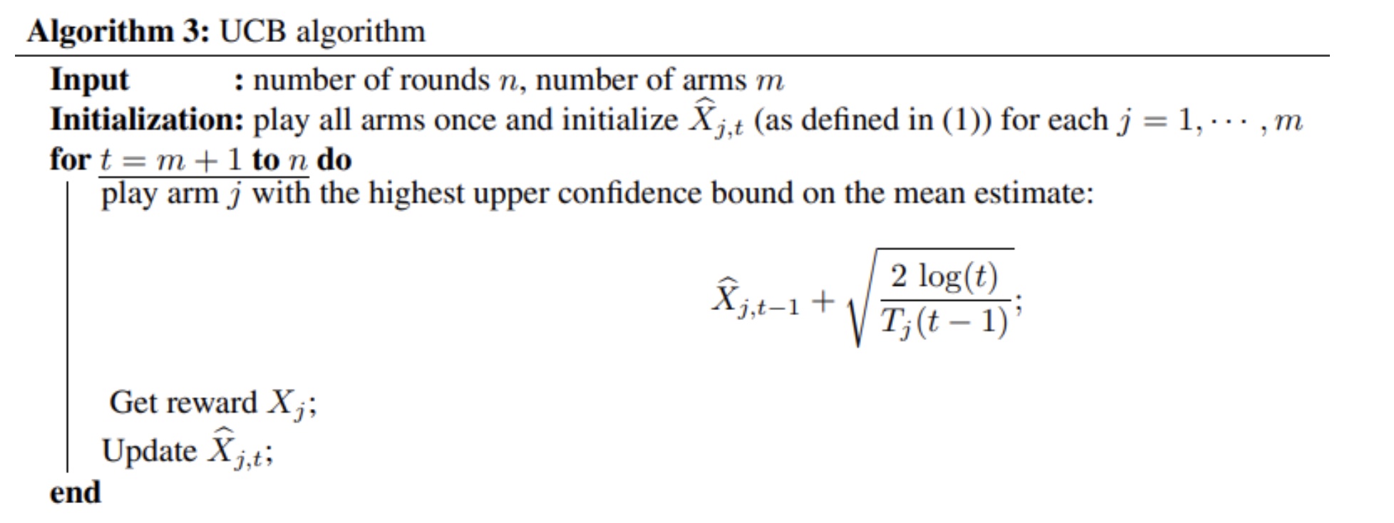
Here’s the classic UCB algorithm (shamelessly stolen from these notes):

Let’s dissect it:

The number of rounds \(n\) is the total number of steps. The gambler is going to choose an arm \(n\) times. There are \(m\) arms. \(\hat{X}_{j, t}\) is the average reward measured for arm \(j\) at step \(t\). Initial values for each arm (\(\hat{X}_{1, 0}\), \(\hat{X}_{2, 0}\), …, \(\hat{X}_{m, 0}\)) are obtained by playing each arm once at the beginning. \(\hat{X}_{j, t-1}\) is the average reward measured for arm \(j\) at step \(t-1\). The sum \(\hat{X}_{j, t-1} + \sqrt{\frac{2log(t)}{T_j(t-1)}}\) is the mean value plus an exploration term.

This is how the classic implementation manages the trade-off between exploration and exploitation:

• The mean reward takes care of the exploitation part.
• The \(T_j(t-1)\) term increases as you select the same arm. Naturally, the uncertainty on the average value decreases (the standard deviation of mean is equal to the standard deviation of the population divided by \(\sqrt{n}\) in the frequentist frame). For arms that haven’t been selected as many times, their uncertainty remains high which increases their chances to be picked up because the upper confidence bound remains high, which leaves space for exploration.
• In the exploration term, \(T_j(t-1)\) is the number of times arm \(j\) was selected in the past steps. It ensures that the arms that have been played the most have a lower exploration term, and that other arms are given higher priority.

Note: some implementations use \(log(t-1)\) instead of \(2log(t)\). In the former, the UCB is “tighter” which reduces the exploration rate. This is known as the UCB1 variation.

Bayes-UCB algorithm

In their paper On Bayesian Upper Confidence Bounds for Bandit Problems, Emilie Kaufmann, Olivier Cappé et Aurélien Garivier propose a Bayes version of the UCB algorithm. In a nutshell, the difference between the “frequentist” and the Bayesian approach lies in the definition of the mean reward. In the former, it is an unknown but fixed quantity that we estimate by computing an average and in the latter, a probability distribution.

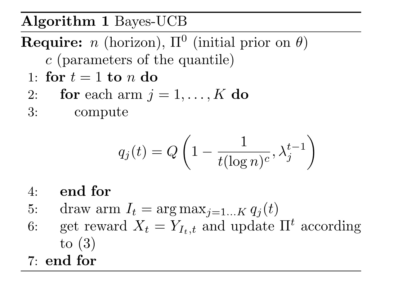
Theorems and lemmas aside, here’s what we can learn by looking directly at the algorithm. The notation is different from the previous algorithm:

The horizon \(n\) is also the total number of steps. \(\Pi^0\) is the initial prior on the set of the arms’ parameters \(\theta\). In the binary case, they are typically Beta distributions, and in the continuous case, Gaussian distributions (the Bayes-UCB paper uses uninformative priors but the chemistry paper uses an implementation with Gaussian priors). \(c\) designates mysterious “parameters of the quantile”.

The double loop is equivalent to the for loop in the first algorithm: for each time step t, we are computing a quantity \(q_j(t)\) for each arm \(j\) and picking the arm that maximizes this quantity. Here also, the reward \(X_t\) is then sampled from the selected arm. This new data is used to update the posterior distribution \(\Pi^t\), and more specifically the distribution of arm j \(\pi_j^t\), since the arms are assumed to be independent from each other.

Let’s look at \(q_j(t)\) in more detail:

As explained in the paper, \(Q(\alpha, \rho)\) is the quantile function of the distribution \(\rho\). Here the distribution is \(\lambda_j^{t-1}\), the distribution of the arm’s mean reward before the update. We’re looking for the quantile at percentile \(1 - \frac1{t(log n)^c}\), which is another way of defining an Upper Confidence Bound of the current arm’s parameter distribution. The percentile \(1 - \frac1{t(log n)^c}\) is an “artifact of the theoretical analysis [..] But in simulations, the choice c = 0 actually proved to be the most satisfying”. Ok, we’ll assume that. Please replace \(1 - \frac1{t(log n)^c}\) by \(1 - \frac1{t}\) in your head :)

So how is the exploitation-exploration managed in this new implementation?

Bayesian considerations

The reward distribution \(\pi_{j,t}\) is updated using Bayes’ theorem: \(\pi_{j,t} (\theta_j) \propto \nu_{\theta_j}(X_t) \pi_{j,t} (\theta_j)\) where \(\nu_{\theta_j}(X_t)\) is the likelihood of observing reward \(X_t\) given mean \(\theta_j\).

The distribution \(\lambda_{j,t}\) of the mean can be derived from the reward distribution \(\pi_{j,t}\) using Bayes’ theorem, since the mean is a parameter of the reward distribution:

In the case of binary rewards (pass or fail), the reward can be modeled by a Bernoulli random variable with parameter \(\theta\). In order to save ourselves complexity, we can use a Beta distribution for parameter \(\theta\) as a conjugate prior such that \(\theta \sim Beta(a, b)\). The posterior becomes \(Beta(a + S_t(j), b + N_t(j) - S_t(j))\) where \(S_t(j)\) is the sum of rewards collected from that arm until step \(t\), and \(N_t(j)\) is the number of times arm \(j\) was picked up until step \(t\). The quantile is easily computed from this well-known distribution. In the chemistry paper, binary rewards are used for reactivity threshold (the selected conditions are either below or above that threshold).

In the case of continuous reward, we can model it as a Gaussian distribution. Assuming a Gaussian prior, and assuming both the mean and variance of the prior are unknown, we can the following convenient conjugate priors: \(\mu | \sigma_0 \sim \mathcal{N}(\mu_0, \sigma^2/\kappa_0)\) and \(\sigma^2 \sim Inv-Gamma(\alpha_0, \beta_0)\). The resulting posterior is:

where the updated parameters are given by:

\(\kappa_n=\kappa_0+n\), \(\mu_n=\frac{\kappa_0 \mu_0+n \bar{x}}{\kappa_0+n}\), \(\alpha_n=\alpha_0+\frac{n}{2}\) and \(\beta_n=\beta_0+\frac{1}{2}\left[\sum_{i=1}^n\left(x_i-\bar{x}\right)^2+\frac{\kappa_0 n\left(\bar{x}-\mu_0\right)^2}{\kappa_0+n}\right]\).

Once again, all distributions are well-known and the quantiles are ready to be inferred.

In the chemistry paper, the authors actually did something simpler and used a fixed variance:

class BayesUCBGaussianPPF(UCB1):
    # Used to be called NewBayesUCBGaussian
    # same as BayesUCBBetaPPF, but uses a gaussian prior with fixed variance

    def __str__(self):
        return f'bayes_ucb_gaussian_ppf'

    def update(self, chosen_arm, reward):
        RegretAlgorithm.update(self, chosen_arm, reward)
        stds = [1 / math.sqrt(c + 1) for c in self.counts]
        self.ucbs = [norm.ppf((1-1/sum(self.counts)), m, s) for m, s in zip(self.emp_means, stds)]

Quick word about the UCB1-tuned algorithm:

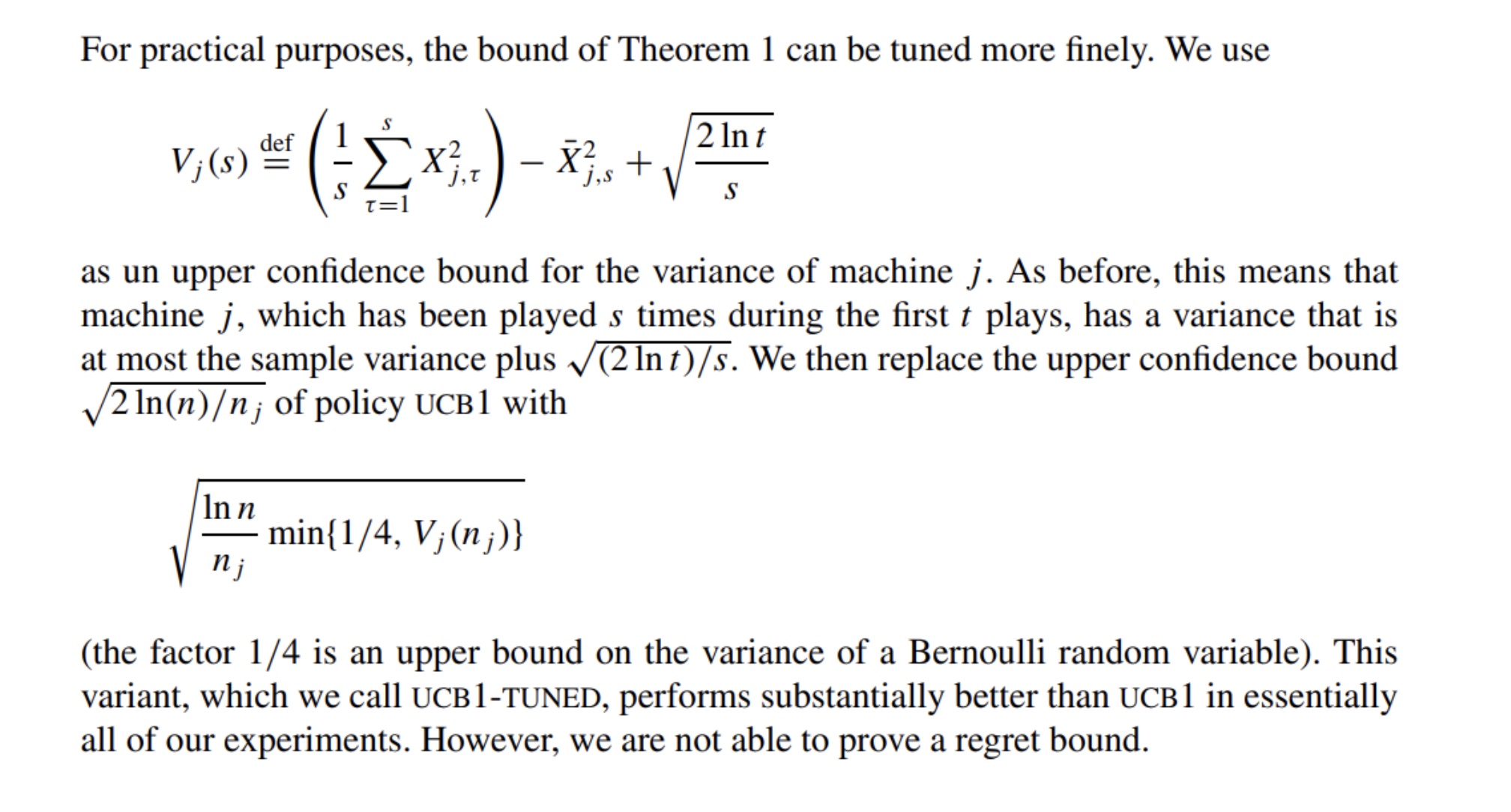
This algorithm is also being used in the paper and is a variation of the UCB algorithm. Contrary to UCB and Bayes-UCB, it takes into account the measured variance. The UCB1-Tuned has also the advantage of not requiring user-defined parameters, although being slightly less performant as the Bayes-UCB.

Here’s an extract from the original paper:

Sources:

https://www.nature.com/articles/s41586-024-07021-y

https://github.com/doyle-lab-ucla/bandit-optimization

https://towardsdatascience.com/multi-armed-bandits-upper-confidence-bound-algorithms-with-python-code-a977728f0e2d

https://link.springer.com/article/10.1023/A:1013689704352

https://proceedings.mlr.press/v22/kaufmann12/kaufmann12.pdf

https://users.cs.duke.edu/~cynthia/CourseNotes/MABNotes.pdf

https://webdocs.cs.ualberta.ca/~games/go/seminar/notes/2007/slides_ucb.pdf