Decision trees in 6 minutes

After 2 years of doing projects in the machine learning space, I realized I didn’t know how decision tree models actually worked. I never felt the urge of learning the inner working for 2 reasons:

• My early ML classes focused on differentiable models (Andrew Ng).
• Implementation of decision trees with the Python scikit-learn, is very easy and high-level.

So, I decided to take a good look! This short post contains a quick description of the training process of a decision tree in a language my future self will understand, and hopefully you too.

I. The tree structure

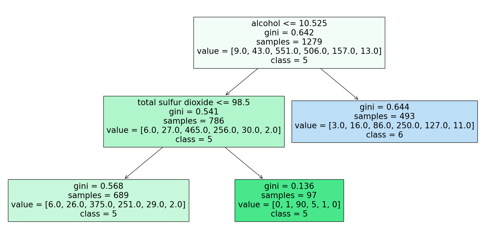
I’m sure you’ve encountered tree structures before, and they’re fairly easy to make sense of when presented in that format: take your input, and depending on its features (alcohol content, sulfur dioxide content), follow the path. Boom. Your output (in this case, your wine quality) is predicted to be a 6 (good) or a 5 (less good). Straightforward.

But this tree is just one tree among a myriad of possibilities, and I could come up with an infinity of combinations: why not sort wines based on their density instead of their alcohol content at the root node? Why not change the threshold to 2.120 instead of 10.525? What decided that structure and these specific sequence of features and thresholds? Let’s break it down:

At every node (nodes represent stages at which data gets sorted) of the tree, we want to separate the training data into different groups in a fashion that allows us to retrieve more homogeneous subsets (in terms of their target variable) at every step. In the case of classification (resp. regression), this means that training points with similar labels (resp., target values) tend to get sorted in the same subset.

In order to determine what feature will be used to separate the data, and what threshold will be used, the algorithm loops through all possible (feature, threshold) combinations, computes a criterion metric (information gain, Gini impurity, variance reduction) every time and picks the combination that optimizes that metric. This criterion metrics assess how much the separation homogenized the new subsets with respect to the initial one.

Let’s take the information gain as an example:

Without diving into too much details, the information gain is a metric used in classification problems, which works well with the wine quality dataset (wines are classified into 6 quality categories: 3, 4, 5, 6, 7, and 8). If you’re a bit familiar with Shannon’s entropy (\(H = - \sum_{i} p_i \log_{2}(p_i)\)), it’s fairly easy to understand:

where \(X\), \(X_1\) and \(X_2\) represent the initial dataset, first and second subsets. We gain information when the entropies of subsets 1 and 2 are lower than the entropy of the dataset before separation. In other words, the distribution of points in these subsets tends to be more concentrated around one class compared to the previous dataset’s distribution.

So with information gain, we have a quantitative ways of assessing what (feature, threshold) combination returns the most informative separation at each node. I leave you with this intuition, but I encourage you to check the math behind the other metrics as well!

If you keep doing that process at every node, you’ll end up with a beautiful tree structure. Now, there are hyperparameters you can adjust to restrict the arborescence of the tree and avoid overfitting. Setting a maximum depth, and setting a minimum information gain are ways to go.

II. Inference

Inference consist in running your sample from the root node to until it reaches terminal node. For classification, we typically classify the sample in the class that is the most represented in the corresponding training subset. If the majority of training points are from class 6, the test point gets attributed the class 6. For regression, we would take the average of training points’ target value as the predicted value.

In the wine quality dataset, features are continuous (alcohol content, total sulfur dioxide content…). But we could have features that are categorical (e.g., color). In that case, we would loop through every (feature, feature category) combinations.

This is the code I used to generate the figure:

import pandas as pd
from sklearn.model_selection import train_test_split
from sklearn.tree import DecisionTreeClassifier
from sklearn import tree
import matplotlib.pyplot as plt

# Load the dataset
url = "https://archive.ics.uci.edu/ml/machine-learning-databases/wine-quality/winequality-red.csv"
data = pd.read_csv(url, delimiter=';')

# Separate features and target variable
X = data.drop('quality', axis=1)
y = data['quality']

# Split the dataset into training and test sets
X_train, X_test, y_train, y_test = train_test_split(X, y, test_size=0.2, random_state=42)

# Train a decision tree classifier
clf = DecisionTreeClassifier(random_state=42, max_depth=3, max_leaf_nodes=3)
clf.fit(X_train, y_train)

# Plot the decision tree
plt.figure(figsize=(20, 10))
tree.plot_tree(clf, filled=True, feature_names=X.columns, class_names=['3', '4', '5', '6', '7', '8'])
plt.show()

Sources:

https://en.wikipedia.org/wiki/Decision_tree_learning

https://towardsdatascience.com/decision-trees-explained-3ec41632ceb6