Gaussian Processes

Introduction

My recent reflection on uncertainty quantification in machine learning led me to take a closer look at Gaussian Processes. Turns out that Gaussian processes inherently allow us to compute some kind of uncertainty!

Bayesian Perspective on Weight Derivation

What most machine learning models do is come up with a set of weights or a model we can use to do inference. Usually, the way these weights are derived is by looking at the Maximum A Posteriori (MAP), which means they maximize the posterior distribution. If you look at the Bayesian interpretation of ordinary least squares or ridge regression, it turns out that it is equivalent to finding the weights that maximize the weights’ posterior distribution.

\[\hat{\theta} = \arg\max_\theta P(\theta | X, Y) = \arg\max_\theta P(Y | X, \theta) P(\theta)\]

Posterior Predictive Distribution

But the problem with this approach is that you only consider a single set of weights for your predictions. And in the process, you ruled out completely other possible models, although they may be as valid! Gaussian processes allow us to take into account all model configurations by directly modeling the posterior predictive distribution. Indeed, if we look at it from the Bayesian perspective, we see that the posterior predictive distribution integrates over all possible sets of model weights:

\[P(Y^* | X^*, X, Y) = \int_{\theta} P(Y^* | X^*, \theta) P(\theta | X, Y) d\theta\]

Assumption of Gaussian Distributions

The idea behind Gaussian processes is to assume that the posterior predictive distribution is a multivariate Gaussian. This video explains nicely why this assumption is reasonable. Here is the short version: if your prior and your likelihood distributions are assumed to be Gaussian, then the posterior distribution becomes Gaussian immediately (because Gaussian distributions are conjugate prior of… Gaussian distributions).

\[P(Y | X) \sim \mathcal{N}(\mu, \Sigma)\]

Covariance Matrix and Kernel Trick

The Gaussian distribution assumption is reasonable and we’ll go on with it. Now here’s the trick: not only do we assume that the training set follows a Gaussian distribution, we also assume that the combination of the training points and the test points also follow a multivariate Gaussian distribution:

\[\begin{bmatrix} Y \\ Y^* \end{bmatrix} \sim \mathcal{N} \left( \begin{bmatrix} \mu \\ \mu^* \end{bmatrix}, \Sigma \right)\]

What should our Gaussian distribution parameters (mean values and covariance matrix) be? It turns out we don’t really care about the mean values. The simple, practical explanation is that we can center the data around zero as a preprocessing step. Regarding the covariance matrix, we can use a cool trick: a kernel! Essentially, a kernel enables us to define a surrogate for the covariance matrix which is more a “similarity matrix” than it is a covariance matrix.

\[\Sigma = \begin{bmatrix} K_{X, X} & K_{X, X^*} \\ K_{X, X^*}^T & K_{X^*, X^*} \end{bmatrix}\]

where \(K_{X, X}\) is the train covariance matrix, \(K_{X, X^*}\) is the train-test covariance matrix and \(K_{X^*, X^*}\) the test covariance matrix.

The RBF kernel is commonly used and is a way to capture the similarity between two data points:

\[k(x, x') = \sigma_f^2\exp\left(-\frac{\|x - x'\|^2}{2l}\right)\]

Note that this expression can be generalized when the input space has several dimensions: \(k(x, x') = \sigma_f^2\exp\left(-\frac1{2l}(\textbf{x} - \textbf{x'})^T(\textbf{x} - \textbf{x'})\right)\)

“But why the heck are we customizing the covariance matrix?”

Well, there is no way we can come up with a meaningful covariance matrix given our current dataset. What would it even mean to compute a variance between \(y_1\) and \(y_n\)? They’re single observations! However, we can use a kernel function to compute the similarity between the corresponding input values. And in return, these can lead to a surrogate to the covariance matrix in the joint distribution that captures this simple idea: if two input values \(x\) and \(x'\) are similar, then the associated output values \(y\) and \(y'\) should be similar too! The best way to grasp this is to take a look at a slice from a 2D-Gaussian distribution where the two components are correlated. If one moves, the other moves too, hence the high “covariance”.

By choosing an appropriate kernel function that correctly captures the similarity between input values, we should retrieve a nice joint distribution. Now, we need to derive the conditional distribution of the test point we want to infer. Here’s the formula, I’m sparing myself the math:

\[P(Y^* | X^*, X, Y) \sim \mathcal{N}(K_{X^*, X} K_{X, X}^{-1} Y, K_{X^*, X^*} - K_{X^*, X} K_{X, X}^{-1} K_{X, X^*})\]

Some intuition

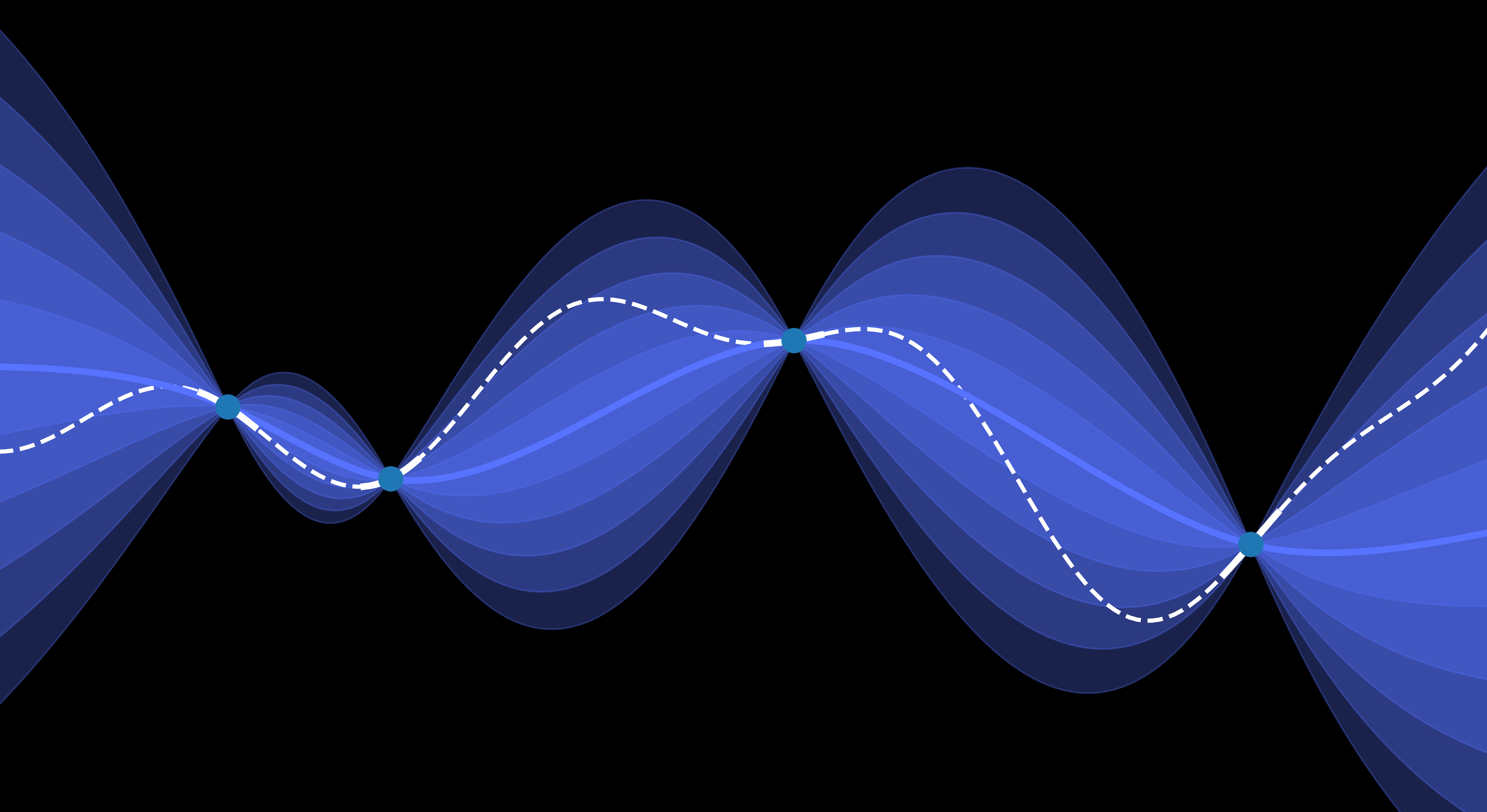
What’s important to understand at this point is that candidate “functions” that model our data can be sampled from the joint distribution. I used quote marks here because we don’t retrieve a function per se, but rather a set of what the true values could look like for the different \(x\) values. If I have 20 points in my training set, I am basically sampling one vector from a 20-dimnensional Gaussian distribution. This is well explained in this short paper.

In addition, the joint distribution and its kernel constitute a prior (“kernelized prior function”), and the conditional distribution is the posterior distribution we obtain by acknowledging the training data (\(Y\) vector).

Hyperparameter Optimization

The kernel function we introduced has two parameters \(\sigma_f\) and \(l\), respectively the vertical and horizontal scale. I’ll designated them under the term \(\beta\). They can be optimized by maximizing the log marginal likelihood \(\log P(Y \| X, \beta)\) (it’s almost the same multivariate distribution we used earlier, but without the test points):

\[\beta^* = \arg\max_\beta \log P(Y|X,\beta) = \arg\max_\beta -\frac1{2}Y^TK^{-1}Y - \frac{n}{2}\log2\pi -\frac1{2}\log|K|\]

Conclusion

This is only the beginning of my exploration with Gaussian processes, and I’m eager to learn more about the applications. My understanding is that Gaussian processes are well suited for small datasets but scale badly with big datasets, especially because matrix inversion has a computation time complexity of \(O(n^3)\). However, I am really hyped about the uncertainty measure we can get out of it.

Sources

https://www.cs.cornell.edu/courses/cs4780/2018fa/lectures/lecturenote15.html

https://scikit-learn.org/stable/modules/gaussian_process.html

https://en.wikipedia.org/wiki/Gaussian_process

https://www.youtube.com/watch?v=UBDgSHPxVME

https://arxiv.org/pdf/2009.10862